Student Alcoholic

알콜중독 학생 분석

• 결론 : 당연한 결과가 나온 것 같음.
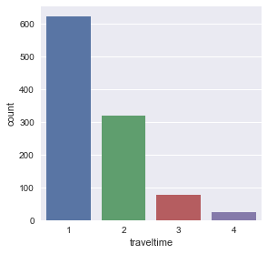
• 집과 학교가 거리가 멀고, 친구들과 밖으로 자주 놀러 나가는 남자 아이가 술을 먹을 확률이 높다.
• 주중에 먹는애가 주말에 먹고, 주말에 먹는 아이가 주중에 먹을 확률 또한 높다. (당연한 소리)
• 결석을 자주하는 아이 또한 가능성은 있지만 높은 편은 아니다.

Attributes for both student-mat.csv (Math course) and student-por.csv (Portuguese language course) datasets:

• school - student’s school (binary: ‘GP’ - Gabriel Pereira or ‘MS’ - Mousinho da Silveira)
• sex - student’s sex (binary: ‘F’ - female or ‘M’ - male)
• age - student’s age (numeric: from 15 to 22)
• address - student’s home address type (binary: ‘U’ - urban or ‘R’ - rural)
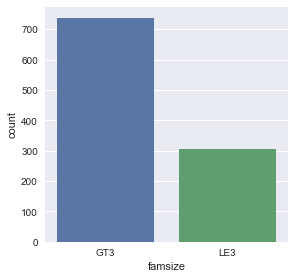
• famsize - family size (binary: ‘LE3’ - less or equal to 3 or ‘GT3’ - greater than 3)
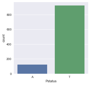
• Pstatus - parent’s cohabitation status (binary: ‘T’ - living together or ‘A’ - apart)
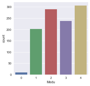
• Medu - mother’s education (numeric: 0 - none, 1 - primary education (4th grade), 2 – 5th to 9th grade, 3 – secondary education or 4 – higher education)
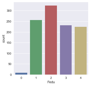
• Fedu - father’s education (numeric: 0 - none, 1 - primary education (4th grade), 2 – 5th to 9th grade, 3 – secondary education or 4 – higher education)
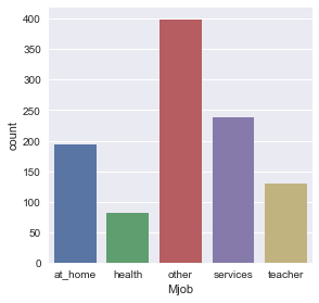
• Mjob - mother’s job (nominal: ‘teacher’, ‘health’ care related, civil ‘services’ (e.g. administrative or police), ‘at_home’ or ‘other’)
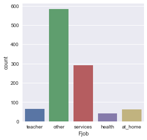
• Fjob - father’s job (nominal: ‘teacher’, ‘health’ care related, civil ‘services’ (e.g. administrative or police), ‘at_home’ or ‘other’)
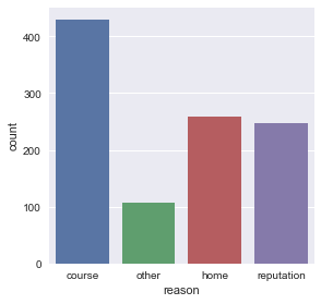
• reason - reason to choose this school (nominal: close to ‘home’, school ‘reputation’, ‘course’ preference or ‘other’)
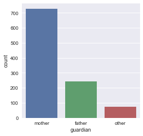
• guardian - student’s guardian (nominal: ‘mother’, ‘father’ or ‘other’)
• traveltime - home to school travel time (numeric: 1 - <15 min., 2 - 15 to 30 min., 3 - 30 min. to 1 hour, or 4 - >1 hour)
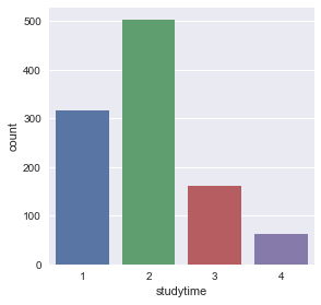
• studytime - weekly study time (numeric: 1 - <2 hours, 2 - 2 to 5 hours, 3 - 5 to 10 hours, or 4 - >10 hours)
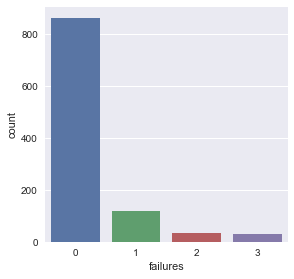
• failures - number of past class failures (numeric: n if 1<=n<3, else 4)
• schoolsup - extra educational support (binary: yes or no)
• famsup - family educational support (binary: yes or no)
• paid - extra paid classes within the course subject (Math or Portuguese) (binary: yes or no)
• activities - extra-curricular activities (binary: yes or no)
• nursery - attended nursery school (binary: yes or no)
• higher - wants to take higher education (binary: yes or no)
• internet - Internet access at home (binary: yes or no)
• romantic - with a romantic relationship (binary: yes or no)
• famrel - quality of family relationships (numeric: from 1 - very bad to 5 - excellent)
• freetime - free time after school (numeric: from 1 - very low to 5 - very high)
• goout - going out with friends (numeric: from 1 - very low to 5 - very high)
• Dalc - workday alcohol consumption (numeric: from 1 - very low to 5 - very high)
• Walc - weekend alcohol consumption (numeric: from 1 - very low to 5 - very high)
• health - current health status (numeric: from 1 - very bad to 5 - very good)
• absences - number of school absences (numeric: from 0 to 93)

these grades are related with the course subject, Math or Portuguese:

• G1 - first period grade (numeric: from 0 to 20)
• G2 - second period grade (numeric: from 0 to 20)
• G3 - final grade (numeric: from 0 to 20, output target)

import pandas as pd
import numpy as np
import matplotlib.pyplot as plt
import seaborn as sns
import datetime as dt

%matplotlib inline

df1 = pd.read_csv("data/student-mat.csv") # 수학
df2 = pd.read_csv("data/student-por.csv") # 포르투칼어

df1['class'] = 'math'
df2['class'] = 'por'

df = df1.append(df2)

df.T.iloc[:,1:5]

	1	2	3	4
school	GP	GP	GP	GP
sex	F	F	F	F
age	17	15	15	16
address	U	U	U	U
famsize	GT3	LE3	GT3	GT3
Pstatus	T	T	T	T
Medu	1	1	4	3
Fedu	1	1	2	3
Mjob	at_home	at_home	health	other
Fjob	other	other	services	other
reason	course	other	home	home
guardian	father	mother	mother	father
traveltime	1	1	1	1
studytime	2	2	3	2
failures	0	3	0	0
schoolsup	no	yes	no	no
famsup	yes	no	yes	yes
paid	no	yes	yes	yes
activities	no	no	yes	no
nursery	no	yes	yes	yes
higher	yes	yes	yes	yes
internet	yes	yes	yes	no
romantic	no	no	yes	no
famrel	5	4	3	4
freetime	3	3	2	3
goout	3	2	2	2
Dalc	1	2	1	1
Walc	1	3	1	2
health	3	3	5	5
absences	4	10	2	4
G1	5	7	15	6
G2	5	8	14	10
G3	6	10	15	10
class	math	math	math	math

탐색적 분석

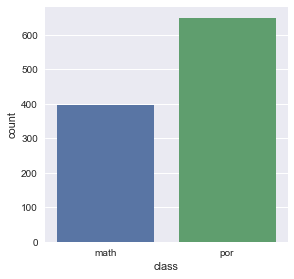
print(df['class'].value_counts())
sns.factorplot('class',kind='count', data=df)

por     649
math    395
Name: class, dtype: int64





<seaborn.axisgrid.FacetGrid at 0x19b19d91748>

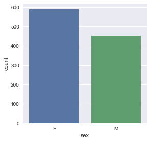
print(df['sex'].value_counts())
sns.factorplot('sex',kind='count', data=df)

F    591
M    453
Name: sex, dtype: int64





<seaborn.axisgrid.FacetGrid at 0x19b19ddf2e8>

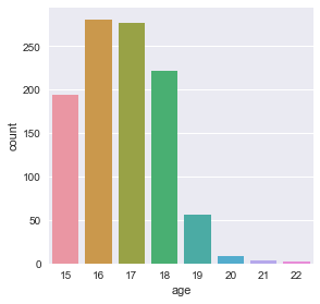
print(df['age'].value_counts())
sns.factorplot('age',data=df, kind='count')

16    281
17    277
18    222
15    194
19     56
20      9
21      3
22      2
Name: age, dtype: int64





<seaborn.axisgrid.FacetGrid at 0x19b19e4f240>

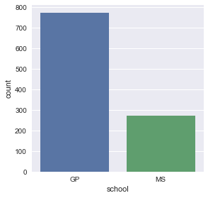
print(df['school'].value_counts())
sns.factorplot('school',kind='count', data=df)

GP    772
MS    272
Name: school, dtype: int64





<seaborn.axisgrid.FacetGrid at 0x19b19e81550>

• GridExtra 처럼 그릴 수 있는 방법이 있을텐데… 찾아봐야됨

sns.factorplot('famsize',kind='count', data=df)
sns.factorplot('Pstatus',kind='count', data=df)
sns.factorplot('Medu',kind='count', data=df)
sns.factorplot('Fedu',kind='count', data=df)
sns.factorplot('Mjob',kind='count', data=df)
sns.factorplot('Fjob',kind='count', data=df)
sns.factorplot('reason',kind='count', data=df)
sns.factorplot('guardian',kind='count', data=df)
sns.factorplot('traveltime',kind='count', data=df)
sns.factorplot('studytime',kind='count', data=df)
sns.factorplot('failures',kind='count', data=df)

<seaborn.axisgrid.FacetGrid at 0x19b1b28bba8>

Finding Correation with Alcol

• 연속형 변수와 명목형으로 나누어 명목형은 Dummpy형태로 변환
• 숫자형이 아닐 경우 Correation을 구할 수가 없다.

columns = df.columns
discrete = []
continuous = []
for i in columns:
    if df[i].dtype =='object':
        discrete.append(i)
    else:
        continuous.append(i)

print(discrete)

['school', 'sex', 'address', 'famsize', 'Pstatus', 'Mjob', 'Fjob', 'reason', 'guardian', 'schoolsup', 'famsup', 'paid', 'activities', 'nursery', 'higher', 'internet', 'romantic', 'class']

print(continuous)

['age', 'Medu', 'Fedu', 'traveltime', 'studytime', 'failures', 'famrel', 'freetime', 'goout', 'Dalc', 'Walc', 'health', 'absences', 'G1', 'G2', 'G3']

dummy = pd.get_dummies(df[discrete])

dummy.head(3)

	school_GP	school_MS	sex_F	sex_M	address_R	address_U	famsize_GT3	famsize_LE3	Pstatus_A	Pstatus_T	...	nursery_no	nursery_yes	higher_no	higher_yes	internet_no	internet_yes	romantic_no	romantic_yes	class_math	class_por
0	1	0	1	0	0	1	1	0	1	0	...	0	1	0	1	1	0	1	0	1	0
1	1	0	1	0	0	1	1	0	0	1	...	1	0	0	1	0	1	1	0	1	0
2	1	0	1	0	0	1	0	1	0	1	...	0	1	0	1	0	1	1	0	1	0

3 rows × 45 columns

• 데이터 결합.

X = pd.concat([df[continuous], dummy], axis=1)

X.head()

	age	Medu	Fedu	traveltime	studytime	failures	famrel	freetime	goout	Dalc	...	nursery_no	nursery_yes	higher_no	higher_yes	internet_no	internet_yes	romantic_no	romantic_yes	class_math	class_por
0	18	4	4	2	2	0	4	3	4	1	...	0	1	0	1	1	0	1	0	1	0
1	17	1	1	1	2	0	5	3	3	1	...	1	0	0	1	0	1	1	0	1	0
2	15	1	1	1	2	3	4	3	2	2	...	0	1	0	1	0	1	1	0	1	0
3	15	4	2	1	3	0	3	2	2	1	...	0	1	0	1	0	1	0	1	1	0
4	16	3	3	1	2	0	4	3	2	1	...	0	1	0	1	1	0	1	0	1	0

5 rows × 61 columns

corr = X.corr()

corr

	age	Medu	Fedu	traveltime	studytime	failures	famrel	freetime	goout	Dalc	...	nursery_no	nursery_yes	higher_no	higher_yes	internet_no	internet_yes	romantic_no	romantic_yes	class_math	class_por
age	1.000000	-0.130196	-0.138521	0.049216	-0.007870	0.282364	0.007162	0.002645	0.118510	0.133453	...	0.046846	-0.046846	0.244601	-0.244601	0.033229	-0.033229	-0.173800	0.173800	-0.018790	0.018790
Medu	-0.130196	1.000000	0.642063	-0.238181	0.090616	-0.187769	0.015004	0.001054	0.025614	0.001515	...	-0.149287	0.149287	-0.206551	0.206551	-0.249728	0.249728	0.008685	-0.008685	0.101246	-0.101246
Fedu	-0.138521	0.642063	1.000000	-0.196328	0.033458	-0.191390	0.013066	0.002142	0.030075	-0.000165	...	-0.104681	0.104681	-0.191956	0.191956	-0.170012	0.170012	0.039906	-0.039906	0.094795	-0.094795
traveltime	0.049216	-0.238181	-0.196328	1.000000	-0.081328	0.087177	-0.012578	-0.007403	0.049740	0.109423	...	0.018641	-0.018641	0.081857	-0.081857	0.169485	-0.169485	-0.013603	0.013603	-0.079881	0.079881
studytime	-0.007870	0.090616	0.033458	-0.081328	1.000000	-0.152024	0.012324	-0.094429	-0.072941	-0.159665	...	-0.056817	0.056817	-0.186556	0.186556	-0.049695	0.049695	-0.038435	0.038435	0.060934	-0.060934
failures	0.282364	-0.187769	-0.191390	0.087177	-0.152024	1.000000	-0.053676	0.102679	0.074683	0.116336	...	0.083027	-0.083027	0.284893	-0.284893	0.074263	-0.074263	-0.076042	0.076042	0.083043	-0.083043
famrel	0.007162	0.015004	0.013066	-0.012578	0.012324	-0.053676	1.000000	0.136901	0.080619	-0.076483	...	-0.024599	0.024599	-0.041502	0.041502	-0.065972	0.065972	0.051891	-0.051891	0.007091	-0.007091
freetime	0.002645	0.001054	0.002142	-0.007403	-0.094429	0.102679	0.136901	1.000000	0.323556	0.144979	...	0.013837	-0.013837	0.086824	-0.086824	-0.061016	0.061016	-0.012372	0.012372	0.025949	-0.025949
goout	0.118510	0.025614	0.030075	0.049740	-0.072941	0.074683	0.080619	0.323556	1.000000	0.253135	...	-0.013779	0.013779	0.062837	-0.062837	-0.083766	0.083766	-0.003606	0.003606	-0.032011	0.032011
Dalc	0.133453	0.001515	-0.000165	0.109423	-0.159665	0.116336	-0.076483	0.144979	0.253135	1.000000	...	0.080647	-0.080647	0.112964	-0.112964	-0.039511	0.039511	-0.045311	0.045311	-0.011335	0.011335
Walc	0.098291	-0.029331	0.019524	0.084292	-0.229073	0.107432	-0.100663	0.130377	0.399794	0.627814	...	0.084874	-0.084874	0.087271	-0.087271	-0.043615	0.043615	0.016426	-0.016426	0.004043	-0.004043
health	-0.029129	-0.013254	0.034288	-0.029002	-0.063044	0.048311	0.104101	0.081517	-0.013736	0.065515	...	0.005869	-0.005869	-0.008036	0.008036	0.041685	-0.041685	0.002096	-0.002096	0.006205	-0.006205
absences	0.153196	0.059708	0.040829	-0.022669	-0.075594	0.099998	-0.062171	-0.032079	0.056142	0.132867	...	0.010842	-0.010842	0.072556	-0.072556	-0.090652	0.090652	-0.105323	0.105323	0.160125	-0.160125
G1	-0.124121	0.226101	0.195898	-0.121053	0.211314	-0.374175	0.036947	-0.051985	-0.101163	-0.150943	...	-0.047878	0.047878	-0.271476	0.271476	-0.104772	0.104772	0.055869	-0.055869	-0.079727	0.079727
G2	-0.119475	0.224662	0.182634	-0.140163	0.183167	-0.377172	0.042054	-0.068952	-0.108411	-0.131576	...	-0.052818	0.052818	-0.250619	0.250619	-0.122517	0.122517	0.097719	-0.097719	-0.126459	0.126459
G3	-0.125282	0.201472	0.159796	-0.102627	0.161629	-0.383145	0.054461	-0.064890	-0.097877	-0.129642	...	-0.039950	0.039950	-0.236578	0.236578	-0.107064	0.107064	0.098363	-0.098363	-0.187166	0.187166
school_GP	-0.169938	0.235114	0.187611	-0.258834	0.133255	-0.066856	0.036359	-0.026008	-0.037000	-0.066006	...	-0.019349	0.019349	-0.131382	0.131382	-0.222993	0.222993	0.074506	-0.074506	0.256088	-0.256088
school_MS	0.169938	-0.235114	-0.187611	0.258834	-0.133255	0.066856	-0.036359	0.026008	0.037000	0.066006	...	0.019349	-0.019349	0.131382	-0.131382	0.222993	-0.222993	-0.074506	0.074506	-0.256088	0.256088
sex_F	0.038832	-0.109387	-0.070786	-0.042508	0.239972	-0.065543	-0.074725	-0.181603	-0.062530	-0.275928	...	-0.030492	0.030492	-0.078775	0.078775	0.062671	-0.062671	-0.108944	0.108944	-0.062192	0.062192
sex_M	-0.038832	0.109387	0.070786	0.042508	-0.239972	0.065543	0.074725	0.181603	0.062530	0.275928	...	0.030492	-0.030492	0.078775	-0.078775	-0.062671	0.062671	0.108944	-0.108944	0.062192	-0.062192
address_R	0.071257	-0.179720	-0.124303	0.343803	-0.037480	0.061160	0.016801	0.009744	-0.030790	0.064030	...	0.031946	-0.031946	0.074716	-0.074716	0.194790	-0.194790	-0.021209	0.021209	-0.087916	0.087916
address_U	-0.071257	0.179720	0.124303	-0.343803	0.037480	-0.061160	-0.016801	-0.009744	0.030790	-0.064030	...	-0.031946	0.031946	-0.074716	0.074716	-0.194790	0.194790	0.021209	-0.021209	0.087916	-0.087916
famsize_GT3	-0.013290	0.025556	0.047290	-0.031550	0.035109	0.044589	0.005328	0.007249	-0.005889	-0.075646	...	0.101279	-0.101279	0.000650	-0.000650	0.008315	-0.008315	-0.007656	0.007656	0.007705	-0.007705
famsize_LE3	0.013290	-0.025556	-0.047290	0.031550	-0.035109	-0.044589	-0.005328	-0.007249	0.005889	0.075646	...	-0.101279	0.101279	-0.000650	0.000650	-0.008315	0.008315	0.007656	-0.007656	-0.007705	0.007705
Pstatus_A	-0.006887	0.077133	0.049156	-0.033883	-0.005049	0.004615	-0.042448	-0.038714	-0.020498	-0.015777	...	-0.054016	0.054016	0.007339	-0.007339	0.065260	-0.065260	-0.050021	0.050021	-0.029497	0.029497
Pstatus_T	0.006887	-0.077133	-0.049156	0.033883	0.005049	-0.004615	0.042448	0.038714	0.020498	0.015777	...	0.054016	-0.054016	-0.007339	0.007339	-0.065260	0.065260	0.050021	-0.050021	0.029497	-0.029497
Mjob_at_home	0.089702	-0.387814	-0.188731	0.170171	-0.018424	0.070264	-0.017289	-0.047825	-0.036958	-0.015903	...	0.025619	-0.025619	0.153985	-0.153985	0.240790	-0.240790	-0.036321	0.036321	-0.073121	0.073121
Mjob_health	-0.093470	0.258135	0.133393	-0.106540	-0.015221	-0.025398	-0.040978	-0.015520	0.046969	-0.076301	...	-0.048189	0.048189	-0.089128	0.089128	-0.088132	0.088132	-0.021277	0.021277	0.021842	-0.021842
Mjob_other	0.037066	-0.231026	-0.200426	0.038616	-0.007451	-0.001451	0.003394	-0.017702	0.006338	-0.004774	...	0.089281	-0.089281	0.021075	-0.021075	0.063474	-0.063474	-0.042049	0.042049	-0.040494	0.040494
Mjob_services	-0.024883	0.104984	0.079390	-0.068560	0.019401	0.058457	0.044812	0.017525	0.031040	0.044716	...	-0.027609	0.027609	-0.035714	0.035714	-0.127412	0.127412	0.056836	-0.056836	0.059108	-0.059108
...	...	...	...	...	...	...	...	...	...	...	...	...	...	...	...	...	...	...	...	...	...
Fjob_at_home	0.065349	-0.091603	-0.084975	-0.052228	0.004087	0.028483	-0.069595	0.045318	-0.023500	-0.029547	...	-0.054813	0.054813	0.068422	-0.068422	0.071043	-0.071043	-0.033594	0.033594	-0.028896	0.028896
Fjob_health	-0.106505	0.128323	0.202267	-0.090635	0.107722	-0.036386	0.003336	-0.039445	0.006843	-0.017665	...	-0.051856	0.051856	-0.044062	0.044062	0.005809	-0.005809	0.016175	-0.016175	0.025293	-0.025293
Fjob_other	0.038894	-0.115679	-0.230861	0.099122	-0.038541	0.007676	0.017535	0.038416	0.043242	-0.060645	...	0.043820	-0.043820	0.001482	-0.001482	0.021934	-0.021934	0.018271	-0.018271	-0.015745	0.015745
Fjob_services	0.001709	-0.019372	0.024698	-0.031258	0.011951	0.031904	0.045152	-0.051199	-0.021470	0.097602	...	0.008235	-0.008235	0.008462	-0.008462	-0.066757	0.066757	0.003417	-0.003417	0.002293	-0.002293
Fjob_teacher	-0.061390	0.260111	0.348978	-0.021649	-0.033607	-0.073646	-0.054509	0.003558	-0.031480	-0.013600	...	-0.010030	0.010030	-0.050270	0.050270	0.004782	-0.004782	-0.024030	0.024030	0.036023	-0.036023
reason_course	0.018524	-0.116806	-0.059851	0.128033	-0.084553	0.098883	-0.005015	0.082123	0.028489	-0.033164	...	0.033645	-0.033645	0.086021	-0.086021	0.103707	-0.103707	-0.004853	0.004853	-0.070995	0.070995
reason_home	-0.002368	0.024313	0.011945	-0.112132	-0.019542	-0.021017	-0.017715	-0.064393	-0.012108	0.045040	...	0.007495	-0.007495	-0.055619	0.055619	-0.063627	0.063627	-0.010746	0.010746	0.052131	-0.052131
reason_other	0.006563	-0.022861	-0.025451	0.040928	-0.097277	-0.007442	0.003139	-0.008310	-0.002354	0.133297	...	0.002981	-0.002981	0.076511	-0.076511	0.043032	-0.043032	-0.050078	0.050078	-0.031532	0.031532
reason_reputation	-0.023719	0.126800	0.075322	-0.063705	0.187202	-0.087729	0.021509	-0.023762	-0.018991	-0.102682	...	-0.048640	0.048640	-0.097860	0.097860	-0.086240	0.086240	0.052339	-0.052339	0.051832	-0.051832
guardian_father	-0.126978	-0.043620	0.094286	0.024526	0.011457	-0.059589	0.008734	-0.032711	-0.064810	0.034565	...	0.018996	-0.018996	-0.022041	0.022041	-0.025185	0.025185	0.049031	-0.049031	-0.009065	0.009065
guardian_mother	-0.081701	0.097703	-0.046298	-0.061961	-0.020958	-0.090476	0.003844	0.003161	0.056714	-0.077368	...	-0.087220	0.087220	-0.052720	0.052720	0.024057	-0.024057	0.024851	-0.024851	-0.010492	0.010492
guardian_other	0.357601	-0.103730	-0.072834	0.070983	0.018770	0.261738	-0.021398	0.048511	0.005225	0.082103	...	0.125651	-0.125651	0.131501	-0.131501	-0.001605	0.001605	-0.126020	0.126020	0.033924	-0.033924
schoolsup_no	0.202824	0.023618	-0.032450	0.033940	-0.070598	-0.002483	0.007634	0.026126	0.051227	0.025852	...	0.028795	-0.028795	0.077115	-0.077115	-0.016827	0.016827	-0.089979	0.089979	-0.037141	0.037141
schoolsup_yes	-0.202824	-0.023618	0.032450	-0.033940	0.070598	0.002483	-0.007634	-0.026126	-0.051227	-0.025852	...	-0.028795	0.028795	-0.077115	0.077115	0.016827	-0.016827	0.089979	-0.089979	0.037141	-0.037141
famsup_no	0.116904	-0.143063	-0.153342	0.026117	-0.143858	0.027574	-0.002261	-0.006227	-0.005252	0.022275	...	0.039921	-0.039921	0.088449	-0.088449	0.082522	-0.082522	-0.009997	0.009997	0.000590	-0.000590
famsup_yes	-0.116904	0.143063	0.153342	-0.026117	0.143858	-0.027574	0.002261	0.006227	0.005252	-0.022275	...	-0.039921	0.039921	-0.088449	0.088449	-0.082522	0.082522	0.009997	-0.009997	-0.000590	0.000590
paid_no	0.027917	-0.161349	-0.118897	0.083679	-0.105704	0.036389	-0.015404	0.034747	0.012943	-0.041919	...	0.053074	-0.053074	0.124097	-0.124097	0.114189	-0.114189	-0.020512	0.020512	-0.473453	0.473453
paid_yes	-0.027917	0.161349	0.118897	-0.083679	0.105704	-0.036389	0.015404	-0.034747	-0.012943	0.041919	...	-0.053074	0.053074	-0.124097	0.124097	-0.114189	0.114189	0.020512	-0.020512	0.473453	-0.473453
activities_no	0.073648	-0.116924	-0.093800	0.025834	-0.078847	0.027500	-0.051574	-0.128601	-0.072236	0.010584	...	0.025370	-0.025370	0.061667	-0.061667	0.072016	-0.072016	0.042559	-0.042559	-0.022794	0.022794
activities_yes	-0.073648	0.116924	0.093800	-0.025834	0.078847	-0.027500	0.051574	0.128601	0.072236	-0.010584	...	-0.025370	0.025370	-0.061667	0.061667	-0.072016	0.072016	-0.042559	0.042559	0.022794	-0.022794
nursery_no	0.046846	-0.149287	-0.104681	0.018641	-0.056817	0.083027	-0.024599	0.013837	-0.013779	0.080647	...	1.000000	-1.000000	0.044429	-0.044429	-0.002605	0.002605	-0.003646	0.003646	0.009498	-0.009498
nursery_yes	-0.046846	0.149287	0.104681	-0.018641	0.056817	-0.083027	0.024599	-0.013837	0.013779	-0.080647	...	-1.000000	1.000000	-0.044429	0.044429	0.002605	-0.002605	0.003646	-0.003646	-0.009498	0.009498
higher_no	0.244601	-0.206551	-0.191956	0.081857	-0.186556	0.284893	-0.041502	0.086824	0.062837	0.112964	...	0.044429	-0.044429	1.000000	-1.000000	0.063407	-0.063407	-0.103002	0.103002	-0.096707	0.096707
higher_yes	-0.244601	0.206551	0.191956	-0.081857	0.186556	-0.284893	0.041502	-0.086824	-0.062837	-0.112964	...	-0.044429	0.044429	-1.000000	1.000000	-0.063407	0.063407	0.103002	-0.103002	0.096707	-0.096707
internet_no	0.033229	-0.249728	-0.170012	0.169485	-0.049695	0.074263	-0.065972	-0.061016	-0.083766	-0.039511	...	-0.002605	0.002605	0.063407	-0.063407	1.000000	-1.000000	0.049882	-0.049882	-0.078377	0.078377
internet_yes	-0.033229	0.249728	0.170012	-0.169485	0.049695	-0.074263	0.065972	0.061016	0.083766	0.039511	...	0.002605	-0.002605	-0.063407	0.063407	-1.000000	1.000000	-0.049882	0.049882	0.078377	-0.078377
romantic_no	-0.173800	0.008685	0.039906	-0.013603	-0.038435	-0.076042	0.051891	-0.012372	-0.003606	-0.045311	...	-0.003646	0.003646	-0.103002	0.103002	0.049882	-0.049882	1.000000	-1.000000	0.034534	-0.034534
romantic_yes	0.173800	-0.008685	-0.039906	0.013603	0.038435	0.076042	-0.051891	0.012372	0.003606	0.045311	...	0.003646	-0.003646	0.103002	-0.103002	-0.049882	0.049882	-1.000000	1.000000	-0.034534	0.034534
class_math	-0.018790	0.101246	0.094795	-0.079881	0.060934	0.083043	0.007091	0.025949	-0.032011	-0.011335	...	0.009498	-0.009498	-0.096707	0.096707	-0.078377	0.078377	0.034534	-0.034534	1.000000	-1.000000
class_por	0.018790	-0.101246	-0.094795	0.079881	-0.060934	-0.083043	-0.007091	-0.025949	0.032011	0.011335	...	-0.009498	0.009498	0.096707	-0.096707	0.078377	-0.078377	-0.034534	0.034534	-1.000000	1.000000

61 rows × 61 columns

알콜 정도

• 주중 알콜 중독정도 (Dalc)
• 주말 알콜 중독정도 (Walc)

pd.DataFrame({'Walc':corr['Walc'], 'Dalc':corr['Dalc']}).T

	age	Medu	Fedu	traveltime	studytime	failures	famrel	freetime	goout	Dalc	...	nursery_no	nursery_yes	higher_no	higher_yes	internet_no	internet_yes	romantic_no	romantic_yes	class_math	class_por
Dalc	0.133453	0.001515	-0.000165	0.109423	-0.159665	0.116336	-0.076483	0.144979	0.253135	1.000000	...	0.080647	-0.080647	0.112964	-0.112964	-0.039511	0.039511	-0.045311	0.045311	-0.011335	0.011335
Walc	0.098291	-0.029331	0.019524	0.084292	-0.229073	0.107432	-0.100663	0.130377	0.399794	0.627814	...	0.084874	-0.084874	0.087271	-0.087271	-0.043615	0.043615	0.016426	-0.016426	0.004043	-0.004043

2 rows × 61 columns

Rel_Dalc = corr['Dalc']
Rel_Walc = corr['Walc']

• 상관계수가 0.1 이상인 변수만 추출 => 절대값을 하는 이유는 특정 변수가 높을 수록 술을 적게 먹는 변수도 찾기 위해서

Rel_Dalc[abs(Rel_Dalc)>0.1]

age                  0.133453
traveltime           0.109423
studytime           -0.159665
failures             0.116336
freetime             0.144979
goout                0.253135
Dalc                 1.000000
Walc                 0.627814
absences             0.132867
G1                  -0.150943
G2                  -0.131576
G3                  -0.129642
sex_F               -0.275928
sex_M                0.275928
reason_other         0.133297
reason_reputation   -0.102682
higher_no            0.112964
higher_yes          -0.112964
Name: Dalc, dtype: float64

Rel_Walc[abs(Rel_Walc)>0.1]

studytime   -0.229073
failures     0.107432
famrel      -0.100663
freetime     0.130377
goout        0.399794
Dalc         0.627814
Walc         1.000000
health       0.106669
absences     0.139703
G1          -0.142401
G2          -0.128114
G3          -0.115740
sex_F       -0.302623
sex_M        0.302623
Name: Walc, dtype: float64

• Index명 추출.

Rel_Col_Dal = Rel_Dalc[abs(Rel_Dalc)>0.1].index.tolist()
Rel_Col_Wal = Rel_Walc[abs(Rel_Walc)>0.1].index.tolist()

Dal_df = X[Rel_Col_Dal]
Wal_df = X[Rel_Col_Wal]

Dal_df.head()

	age	traveltime	studytime	failures	freetime	goout	Dalc	Walc	absences	G1	G2	G3	sex_F	sex_M	reason_other	reason_reputation	higher_no	higher_yes
0	18	2	2	0	3	4	1	1	6	5	6	6	1	0	0	0	0	1
1	17	1	2	0	3	3	1	1	4	5	5	6	1	0	0	0	0	1
2	15	1	2	3	3	2	2	3	10	7	8	10	1	0	1	0	0	1
3	15	1	3	0	2	2	1	1	2	15	14	15	1	0	0	0	0	1
4	16	1	2	0	3	2	1	2	4	6	10	10	1	0	0	0	0	1

Wal_df.head()

	studytime	failures	famrel	freetime	goout	Dalc	Walc	health	absences	G1	G2	G3	sex_F	sex_M
0	2	0	4	3	4	1	1	3	6	5	6	6	1	0
1	2	0	5	3	3	1	1	3	4	5	5	6	1	0
2	2	3	4	3	2	2	3	3	10	7	8	10	1	0
3	3	0	3	2	2	1	1	5	2	15	14	15	1	0
4	2	0	4	3	2	1	2	5	4	6	10	10	1	0

Dal_corr = Dal_df.corr()
Wal_corr = Wal_df.corr()

결론

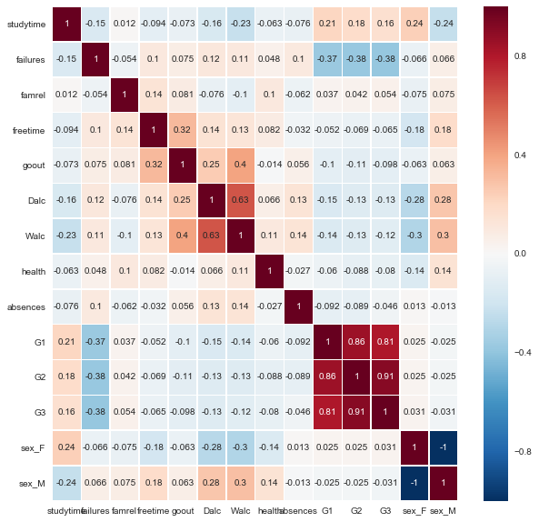
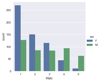
• 남자학생의 경우가 여성의 학생보다 알콜 중독 현상이 높다.
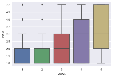
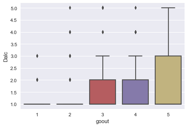
• 당연한 얘기로 밖에 친구와 많이 놀러 가는 학생이 알콜에 노출될 확률이 높으므로 더 많은 섭취 현상을 보였다.
• 자유 시간이 많은 학생이 위와 같은 원인으로 더 많은 노출이 되었다.
• 주중 / 주말 알콜 섭취 비율은 당연히 상관관계가 제일 높았다.
• 결석을 많이 하는 학생 또한 약간의 상관 관계를 가지고 있으나 확정적이지는 않다.

fig, ax = plt.subplots(figsize=(10,10))
sns.heatmap(Dal_corr,
            xticklabels=Dal_corr.columns.values,
            yticklabels=Dal_corr.columns.values,
           annot=True, linewidths=.5, ax=ax)

<matplotlib.axes._subplots.AxesSubplot at 0x19b17c00dd8>

fig, ax = plt.subplots(figsize=(10,10))
sns.heatmap(Wal_corr,
            xticklabels=Wal_corr.columns.values,
            yticklabels=Wal_corr.columns.values,
            annot=True, linewidths=.5, ax=ax)

<matplotlib.axes._subplots.AxesSubplot at 0x19b1779d8d0>

sns.boxplot(x='goout',y='Walc',data=df)

<matplotlib.axes._subplots.AxesSubplot at 0x19b185dddd8>

sns.boxplot(x='goout',y='Dalc',data=df)

<matplotlib.axes._subplots.AxesSubplot at 0x19b186df630>

• 여성의 알콜 중독 비율이 남자학생보다 훨씬 낮다.

sns.factorplot('Walc',kind='count',hue='sex',data=df)

<seaborn.axisgrid.FacetGrid at 0x19b187dc320>

Machine Learning 예측

X[['Walc','Dalc']].head()

	Walc	Dalc
0	1	1
1	1	1
2	3	2
3	1	1
4	2	1

X['Alcohol'] = X['Walc'] + X['Dalc']

X['Alcohol'].head()

0    2
1    2
2    5
3    2
4    3
Name: Alcohol, dtype: int64

ml_df = X.copy()

ml_df['Alcohol'].value_counts()

2     391
3     182
4     159
5     118
6      85
7      49
8      26
10     24
9      10
Name: Alcohol, dtype: int64

from sklearn.utils import shuffle

ml_df = shuffle(ml_df)

ml_df = ml_df.reset_index()

del ml_df['index']

ml_df_columns = ml_df.columns.difference(['Walc','Dalc','Alcohol'])

ml_df_columns

Index(['Fedu', 'Fjob_at_home', 'Fjob_health', 'Fjob_other', 'Fjob_services',
       'Fjob_teacher', 'G1', 'G2', 'G3', 'Medu', 'Mjob_at_home', 'Mjob_health',
       'Mjob_other', 'Mjob_services', 'Mjob_teacher', 'Pstatus_A', 'Pstatus_T',
       'absences', 'activities_no', 'activities_yes', 'address_R', 'address_U',
       'age', 'class_math', 'class_por', 'failures', 'famrel', 'famsize_GT3',
       'famsize_LE3', 'famsup_no', 'famsup_yes', 'freetime', 'goout',
       'guardian_father', 'guardian_mother', 'guardian_other', 'health',
       'higher_no', 'higher_yes', 'internet_no', 'internet_yes', 'nursery_no',
       'nursery_yes', 'paid_no', 'paid_yes', 'reason_course', 'reason_home',
       'reason_other', 'reason_reputation', 'romantic_no', 'romantic_yes',
       'school_GP', 'school_MS', 'schoolsup_no', 'schoolsup_yes', 'sex_F',
       'sex_M', 'studytime', 'traveltime'],
      dtype='object')

X = ml_df[ml_df_columns]

y = ml_df['Alcohol']

print(ml_df.columns)
ml_df.head()

Index(['age', 'Medu', 'Fedu', 'traveltime', 'studytime', 'failures', 'famrel',
       'freetime', 'goout', 'Dalc', 'Walc', 'health', 'absences', 'G1', 'G2',
       'G3', 'school_GP', 'school_MS', 'sex_F', 'sex_M', 'address_R',
       'address_U', 'famsize_GT3', 'famsize_LE3', 'Pstatus_A', 'Pstatus_T',
       'Mjob_at_home', 'Mjob_health', 'Mjob_other', 'Mjob_services',
       'Mjob_teacher', 'Fjob_at_home', 'Fjob_health', 'Fjob_other',
       'Fjob_services', 'Fjob_teacher', 'reason_course', 'reason_home',
       'reason_other', 'reason_reputation', 'guardian_father',
       'guardian_mother', 'guardian_other', 'schoolsup_no', 'schoolsup_yes',
       'famsup_no', 'famsup_yes', 'paid_no', 'paid_yes', 'activities_no',
       'activities_yes', 'nursery_no', 'nursery_yes', 'higher_no',
       'higher_yes', 'internet_no', 'internet_yes', 'romantic_no',
       'romantic_yes', 'class_math', 'class_por', 'Alcohol'],
      dtype='object')

	age	Medu	Fedu	traveltime	studytime	failures	famrel	freetime	goout	Dalc	...	nursery_yes	higher_no	higher_yes	internet_no	internet_yes	romantic_no	romantic_yes	class_math	class_por	Alcohol
0	16	4	4	1	2	0	4	4	2	1	...	1	0	1	0	1	0	1	1	0	2
1	16	1	2	1	2	0	4	4	3	1	...	1	0	1	0	1	1	0	0	1	2
2	16	4	4	1	2	0	4	2	4	2	...	1	0	1	0	1	1	0	1	0	6
3	17	4	4	1	1	0	5	2	3	1	...	1	0	1	0	1	1	0	0	1	3
4	19	2	3	1	3	1	4	1	2	1	...	1	0	1	0	1	0	1	1	0	2

5 rows × 62 columns

y[:5]

0    2
1    2
2    6
3    3
4    2
Name: Alcohol, dtype: int64

데이터 분할

from sklearn.model_selection import train_test_split

X_train, X_test, y_train, y_test = train_test_split(X, y, test_size=0.3, random_state=0)

from sklearn.linear_model import LinearRegression

lm = LinearRegression()

X_train.head()

	Fedu	Fjob_at_home	Fjob_health	Fjob_other	Fjob_services	Fjob_teacher	G1	G2	G3	Medu	...	romantic_no	romantic_yes	school_GP	school_MS	schoolsup_no	schoolsup_yes	sex_F	sex_M	studytime	traveltime
830	3	0	0	1	0	0	14	14	15	4	...	1	0	1	0	1	0	1	0	2	1
172	2	0	0	1	0	0	15	14	15	3	...	0	1	0	1	1	0	1	0	2	2
1005	3	0	0	1	0	0	12	11	12	1	...	0	1	0	1	1	0	0	1	1	2
1013	3	0	0	1	0	0	11	10	10	2	...	1	0	1	0	1	0	1	0	3	1
397	3	0	0	0	1	0	10	10	11	3	...	0	1	1	0	1	0	0	1	2	1

5 rows × 59 columns

lm.fit(X_train, y_train)

LinearRegression(copy_X=True, fit_intercept=True, n_jobs=1, normalize=False)

lm.intercept_ #  절편

-552496061212.00085

lm.coef_ #기울기

array([  1.10681983e-01,   7.62085702e+11,   7.62085702e+11,
         7.62085702e+11,   7.62085702e+11,   7.62085702e+11,
        -1.16823836e-01,   6.91050842e-02,  -3.45437923e-03,
        -1.71508789e-02,  -1.42382326e+10,  -1.42382326e+10,
        -1.42382326e+10,  -1.42382326e+10,  -1.42382326e+10,
        -2.79352456e+09,  -2.79352456e+09,   4.22363281e-02,
        -1.04961259e+10,  -1.04961259e+10,   2.35242131e+09,
         2.35242131e+09,   1.11968994e-01,  -4.36248354e+09,
        -4.36248354e+09,   7.52563477e-02,  -3.29772949e-01,
        -1.10872374e+08,  -1.10872374e+08,   1.12212080e+10,
         1.12212080e+10,   8.78906250e-03,   5.69213867e-01,
        -7.05294877e+09,  -7.05294877e+09,  -7.05294877e+09,
         1.04492188e-01,   8.30723019e+09,   8.30723019e+09,
         5.57260644e+09,   5.57260644e+09,  -6.15471185e+08,
        -6.15471186e+08,   4.73224834e+09,   4.73224834e+09,
        -8.98184669e+10,  -8.98184669e+10,  -8.98184669e+10,
        -8.98184669e+10,   4.35991140e+10,   4.35991140e+10,
        -1.55858529e+11,  -1.55858529e+11,   1.15810618e+10,
         1.15810618e+10,  -1.16088761e+10,  -1.16088761e+10,
        -1.85943604e-01,   1.70471191e-01])

from sklearn.metrics import mean_squared_error

mean_squared_error(y_train,lm.predict(X_train))

2.659151246163943

mean_squared_error(y_test,lm.predict(X_test))

2.4619246322163351

compare_alcohol = pd.DataFrame({'prediction':lm.predict(X_test),'real_value':y_test})

compare_alcohol['prediction'] = round(compare_alcohol['prediction'])

compare_alcohol['diff'] = compare_alcohol['prediction'] - compare_alcohol['real_value']

compare_alcohol['diff'].value_counts()

 1.0    83
 0.0    72
-1.0    54
 2.0    49
-2.0    30
-3.0     8
 3.0     8
 4.0     3
-5.0     3
-4.0     3
 6.0     1
Name: diff, dtype: int64

Classification으로 풀기

from sklearn.ensemble import GradientBoostingClassifier

from sklearn import metrics

gb = GradientBoostingClassifier(n_estimators=3000)

gb.fit(X_train,y_train)

GradientBoostingClassifier(criterion='friedman_mse', init=None,
              learning_rate=0.1, loss='deviance', max_depth=3,
              max_features=None, max_leaf_nodes=None,
              min_impurity_split=1e-07, min_samples_leaf=1,
              min_samples_split=2, min_weight_fraction_leaf=0.0,
              n_estimators=3000, presort='auto', random_state=None,
              subsample=1.0, verbose=0, warm_start=False)

def getResult(y_test,y_pred):
    print(metrics.confusion_matrix(y_test, y_pred))
    print('accurracy:', metrics.accuracy_score(y_test, y_pred))

gb.predict(X_test)

array([ 3,  3,  2,  2,  3,  3,  2,  5,  3,  4,  2,  4,  3,  2,  7,  2,  5,
        2,  5,  2,  2,  2,  4,  2,  2,  6,  2,  5,  2,  6,  5,  2,  2,  7,
        5,  2,  2,  2,  6,  2,  3,  4,  2,  5,  2,  5,  2,  3,  6, 10,  4,
        3,  4, 10,  2,  2,  2,  4,  4,  2,  2,  2,  2,  2,  2,  3,  2,  4,
        4,  4,  3,  2,  3,  3,  2,  2,  2,  2,  6,  2,  5,  2,  5,  3,  3,
        6,  2,  2,  3,  7,  6,  5,  5,  4,  2,  2,  3,  3,  2,  4,  6,  4,
        4,  5,  2,  5,  3,  2,  3,  2,  2,  3,  3,  4,  6,  5,  5,  6,  2,
        2,  8,  2,  6,  5,  2,  3,  2,  6,  2,  5,  2,  2,  3,  6,  4,  3,
        2,  3,  3,  2,  2,  4,  2,  2,  4,  2,  4,  5,  3,  2,  2,  2,  3,
        2,  4,  8,  2,  2,  2,  5,  2,  5,  2,  2,  2,  2,  3,  6,  3,  7,
        6,  2,  2,  3,  2,  8,  4,  2,  2,  2,  4,  2,  6,  6,  2,  2,  2,
        2,  2,  2,  2,  2,  5,  2,  3,  6,  2,  6,  2,  3,  2,  2,  2,  2,
        4,  4,  3,  2,  4,  3,  2,  7,  4,  5,  6,  2,  2,  4,  3,  4,  6,
        3,  2,  7,  3,  4,  5,  2,  2,  3,  2,  6,  4,  3,  6,  3,  2,  2,
        3,  4,  2,  2,  2,  5,  7,  7,  4,  5,  2,  4,  2,  2,  2,  3,  4,
        3,  2,  3,  2,  3,  2,  4,  2,  2,  6,  2,  5,  7,  2,  3,  2,  2,
        4,  5,  2,  2,  5,  4,  3,  3,  2,  2,  3,  4,  7,  2,  3,  2,  3,
        2,  2,  2,  2,  3,  4,  2,  4,  3,  3,  4,  2,  3,  5,  2,  3,  2,
        2,  2,  2,  4,  2,  2,  2,  7], dtype=int64)

getResult(gb.predict(X_test),y_test)

[[86 22 14 14  5  2  0  0  0]
 [14 18 12  9  2  3  0  0  0]
 [ 6  7 25  2  2  0  0  0  1]
 [ 2  3  1 16  2  2  2  0  2]
 [ 3  2  0  2  9  6  1  1  0]
 [ 3  2  0  0  1  5  0  0  0]
 [ 1  0  0  0  0  1  1  0  0]
 [ 0  0  0  0  0  0  0  0  0]
 [ 0  0  1  0  0  0  0  0  1]]
accurracy: 0.512738853503